RESEARCH JOURNAL

Gradient vs Isocratic HPLC: A Practical Guide for Analytical Chemists

Discover the advantages of gradient vs isocratic HPLC methods to enhance your analytical chemistry workflows and optimize sample screening.

If you’re screening an unfamiliar peptide or small-molecule sample, start with a scouting gradient. It’s the fastest way to see the full retention window in one run, and it tells you almost immediately whether the sample actually needs a gradient method or can be simplified down to a stable, isocratic assay. The workflow is three steps: run a broad scouting gradient, evaluate how the peaks occupy that gradient window, then either convert to an isocratic method or lock in and optimize the gradient you already have.

This is squarely a method-development question, not a lab-use question. Everything below concerns analytical characterization, purity verification, and identity confirmation for in-vitro research, the kind of work that supports a lot-specific Certificate of Analysis. Nothing here touches dosing, administration, or any in vivo application.

Key Takeaways

Start method development with a broad scouting gradient, then let peak occupancy across that gradient window tell you whether to convert to isocratic conditions or keep refining the gradient itself.

Point	Details
Start with a scouting gradient	Run a broad 5 to 95 percent gradient first to map retention windows before choosing a final mode.
Use occupancy to decide	Tightly clustered peaks favor isocratic conversion; widely spread peaks favor keeping the gradient.
Watch dwell volume for transfer	Document system dwell volume before moving any gradient method between instruments.
Match detector to mode	Refractive-index detectors generally require isocratic elution regardless of sample complexity.
Confirm identity orthogonally	Pair RP-HPLC purity results with mass spectrometry identity confirmation on every lot-specific COA.

Gradient vs Isocratic HPLC: Side-by-Side Comparison
How Isocratic Elution Behaves on the Column
How Gradient Elution Changes Retention Over Time
When to Choose Gradient or Isocratic HPLC
Building a Method: From Scouting Gradient to Final Elution Mode
Designing Gradients That Actually Transfer Between Systems
Equilibration, Solvent Use, and Reproducibility in Daily Practice
Troubleshooting Gradient and Isocratic Method Problems
Agate Research’s Recommended Verification Workflow
Sources

Gradient vs Isocratic HPLC: Side-by-Side Comparison

The core distinction is simple: isocratic elution holds mobile phase composition constant for the entire run, while gradient elution increases solvent strength over time to pull progressively more retentive analytes off the column faster. That one-line difference cascades into almost every practical decision you’ll make about run time, resolution, and instrument load.

HPLC solvents and vials on lab bench

Isocratic methods reward you with a flat, predictable baseline and reproducible retention times, which is why quality control labs running the same simple assay thousands of times often prefer them. Gradient methods trade some of that simplicity for peak capacity, letting you resolve a wide polarity range in a single run instead of stringing together multiple isocratic segments.

Dimension	Isocratic elution	Gradient elution
Sample complexity	Best for simple mixtures with similar polarity	Handles complex, wide-polarity mixtures
Run time / throughput	Shorter for simple samples, no re-equilibration wait	Often faster overall for complex samples despite equilibration time
Peak capacity / resolution	Limited, especially for late eluters	Higher, resolves more components per run
Solvent consumption / cost	Lower, one mobile phase reservoir	Higher, needs at least two solvents and mixing
Reproducibility / transferability	High, unaffected by dwell volume	More variable, sensitive to system dwell volume
Instrument requirements	Simple isocratic pump acceptable	Needs precise binary/quaternary mixing and low dwell volume
Method-development difficulty	Lower once conditions are scouted	Higher, more parameters to optimize
Late-eluter sensitivity	Poor, broad peaks lose signal-to-noise	Strong, narrower peaks improve detection

A few decision rules cut through most of the back-and-forth:

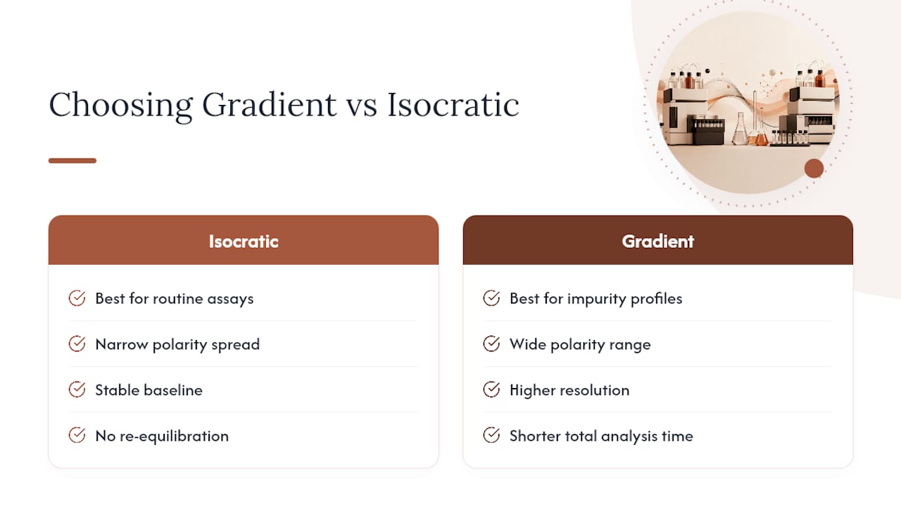
If your analyte physicochemical properties (log D, pKa) cluster tightly, an isocratic method is usually enough.
If you’re running related-substance or impurity-profiling work with a wide polarity spread, gradient elution typically wins on resolution and total analysis time.
If your detector is refractive-index based, gradient elution usually isn’t an option at all, which we’ll get into below.
If you’re transferring a method between labs or instruments with different dwell volumes, isocratic methods travel more predictably.

How Isocratic Elution Behaves on the Column

Isocratic elution keeps the mobile phase composition fixed from injection to detection. Nothing about the solvent strength changes, so the retention mechanism stays constant for every analyte in the run. That constancy is exactly why isocratic baselines are so stable and why integration software has an easy time drawing peak boundaries, since there’s no shifting baseline drift from a changing solvent gradient to compensate for.

The tradeoff shows up with late eluters. Compounds that spend a long time on the column keep diffusing longitudinally the whole time they’re migrating, and under constant mobile phase strength there’s nothing pulling them off faster. The result is broader, flatter peaks with lower signal-to-noise by the time they reach the detector. Picture three peaks from the same isocratic run: an early eluter comes off sharp and tall, a mid-run peak is slightly wider but still crisp, and a late eluter has spread into a shallow hump that’s easy to miss against baseline noise if the concentration is low. That’s diffusion working against you over time, not a defect in the method.

Operationally, isocratic runs are efficient because there’s no need for post-run re-equilibration: the column is already sitting in the mobile phase it needs for the next injection. That efficiency comes at the cost of peak capacity. Cramming a mixture with a wide range of polarities into one isocratic run usually means either the early peaks co-elute or the late peaks disappear into the baseline, sometimes both in the same chromatogram.

Constant composition means constant baseline, which simplifies integration and quantitation.
Predictable retention works well for analytes with similar polarity, like closely related synthetic intermediates.
Late-eluting compounds broaden and lose sensitivity due to extended diffusion time on the column.
No re-equilibration step needed between injections, which helps throughput for routine assays.

Pro Tip: When you’re stuck picking an isocratic mobile phase ratio, run three quick trials bracketing your best guess (say, 5 percentage points apart) rather than one long optimization. Isocratic retention is sensitive enough to small percentage changes that this bracket almost always reveals whether you’re chasing a moving target or genuinely close to optimal.

How Gradient Elution Changes Retention Over Time

Gradient elution deliberately increases mobile phase strength as the run progresses, usually by raising the percentage of organic solvent over time. Early in the run, weakly retained analytes are already moving, while more strongly retained compounds sit tight on the column. As the gradient ramps up, it eventually reaches a solvent strength capable of pulling those later analytes off, and it does so in a narrower band than isocratic conditions would produce, because the compound isn’t sitting still diffusing for nearly as long.

That narrowing band is the whole mechanism behind gradient elution’s sensitivity advantage. Reducing the time a late-eluting analyte spends diffusing on the column improves its signal-to-noise ratio and sharpens what would otherwise be a broad, faint peak into something you can actually integrate with confidence. Peak capacity, the number of resolvable peaks you can fit into a run, goes up correspondingly, which is exactly why gradients dominate in complex mixture work.

Think of gradient shape as a dial you’re turning at different speeds. A shallow, slow-rising gradient behaves almost like an extended isocratic segment for adjacent peaks, giving you more resolution between similar analytes but stretching your run time. A steep gradient compresses everything into a shorter window, which is great for throughput but can crush resolution between components that elute close together. A linear gradient sits in the middle and is usually the default starting point precisely because it’s easy to reason about and easy to reproduce.

None of this comes free on the instrument side. Gradients demand precise solvent mixing, whether that’s a high-pressure binary pump or a low-pressure quaternary system with a mixing chamber, and any imprecision in that mixing directly distorts the apparent gradient the column actually experiences.

Increasing solvent strength over time reduces residence time for late-eluting compounds.
Shorter residence time on column means less diffusion, translating to narrower peaks and better sensitivity.
Peak capacity scales with gradient range, letting you resolve more components per run than isocratic conditions allow.
Shallow gradients favor resolution between similar analytes; steep gradients favor speed.
Precise pump mixing and low dwell volume become essential once you commit to a gradient method.

When to Choose Gradient or Isocratic HPLC

Neither mode is universally better. The right call depends on what your sample actually looks like and what question you’re trying to answer with the chromatogram.

Isocratic methods earn their keep in routine assay work where the analyte and its close relatives share similar polarity, like verifying purity of a single peptide lot against a narrow reference window. The stable baseline and lack of re-equilibration make isocratic runs cheap to repeat hundreds of times, which matters when you’re processing a queue of similar samples rather than exploring an unknown one. Gradient methods make more sense once you’re chasing a related-substance profile or an impurity map where degradation products, synthesis byproducts, or truncated sequences span a much wider polarity range than the parent compound alone. Related-substance and complex impurity work is where gradient elution typically pulls ahead on both resolution and total analysis time, especially for peptide and protein samples where molecular weight and conformation add extra separation challenges beyond simple polarity.

Here’s a worked example of the reasoning, not a protocol: suppose a scouting gradient on a peptide reference standard shows the analyte and its two closest impurities eluting within a tight two-minute window near the middle of the gradient, with nothing else of interest earlier or later. That tight clustering is a signal you can probably convert to isocratic conditions using the mobile phase composition present at the moment those peaks eluted, since the polarity spread across your compounds of interest is narrow enough that a constant composition should resolve them just as well, with a simpler and more transferable method as the payoff. Flip the scenario: if the scout shows peaks scattered across the entire gradient range with real analytical value at both extremes, converting to isocratic would force an impossible tradeoff between resolving the early cluster and detecting the late one, so you stay with a gradient and instead work on optimizing its shape.

Detector compatibility can override all of this reasoning outright. Refractive-index detectors are generally incompatible with gradient elution because the detector reads changes in refractive index against a reference, and a continuously shifting mobile phase composition makes that baseline reference a moving target. If your analytical setup depends on an RI detector, you’re working isocratically by necessity, not preference.

Pro Tip: Before you commit to converting a gradient method to isocratic, check your detector and separation mode against each other first. A mismatch here wastes far more development time than a suboptimal mobile phase ratio ever will.

When to Choose Gradient or Isocratic HPLC — overview diagram

Building a Method: From Scouting Gradient to Final Elution Mode

A disciplined method-development sequence saves you from bouncing between gradient and isocratic trials with no real logic tying them together. This is the order most analytical chemists converge on, whether they started that way or learned it the hard way.

Prepare a broad scouting gradient. Run something like 5 to 95 percent organic modifier over a generous timeframe, wide enough to guarantee every component in your sample elutes somewhere within the window.
Run the scout and record retention times. This single run is the fastest way to map out where every analyte in your mixture actually falls before you commit to a full optimization strategy.
Evaluate peak occupancy across the gradient window. Look at how tightly or how broadly your peaks of interest are distributed across the total run time.
Choose your path. Tightly clustered peaks in a narrow window point toward an isocratic cut; peaks spread across the full range point toward keeping and refining the gradient.

The occupancy rule of thumb is straightforward: if your compounds of interest occupy roughly 10 to 20 percent of the total gradient time in a tight cluster, an isocratic method built around that region’s composition is worth testing. If they’re spread across 50 percent or more of the gradient, you’re almost certainly staying with a gradient method, because no single constant composition will resolve components that differ that much in polarity.

Converting from gradient retention behavior to an isocratic composition is more art than formula, but the general logic holds: the mobile phase strength present at the moment your analytes of interest eluted in the scouting gradient is your starting point for isocratic trials, then you fine-tune from there based on the resolution you actually observe. This is high-level reasoning, not a prescriptive recipe, since actual composition percentages depend heavily on your specific column chemistry and analyte set.

Before calling any method final, run through a robustness checklist:

Confirm column lot-to-lot consistency, since stationary phase batch variation can shift retention independent of your mobile phase.
Check mobile-phase additive concentration and pH control, particularly for ionizable peptide residues where small pH shifts change retention meaningfully.
Verify temperature control, since column oven stability affects both gradient and isocratic retention reproducibility.
Run system suitability injections (replicate precision, resolution between critical pairs, tailing factor) before accepting the method as final.

Pro Tip: Keep your scouting gradient data even after you’ve converted to a final isocratic method. If you ever need to re-evaluate the sample for a new impurity or degradation product down the line, that original scout saves you from starting the whole mapping process over.

Designing Gradients That Actually Transfer Between Systems

Gradient shape isn’t a cosmetic choice. Linear gradients ramp solvent strength at a constant rate and are the default starting point for most method development because they’re the easiest to reason about and the easiest for another lab to reproduce exactly. Step gradients jump abruptly between two or more fixed compositions, useful when you know in advance that your analytes cluster into distinct polarity groups and don’t need a smooth transition between them. Convex and concave (non-linear) gradients accelerate or decelerate the rate of change partway through the run, letting you compress separation time in a region where resolution isn’t critical while stretching it out where it is.

The single biggest threat to transferring any gradient method between instruments is dwell volume, also called gradient delay volume: the volume of mobile phase between where the pump mixes the solvents and where that mixed solvent actually reaches the column. Every LC system has a different dwell volume, and a gradient programmed identically on two different instruments can produce meaningfully different actual gradients at the column inlet if their dwell volumes differ. A method validated on a system with a large dwell volume can shift retention times and resolution when moved to a system with a smaller one, even though every programmed parameter looks identical on paper.

Minimizing the number of segments and inflection points in your gradient profile improves robustness considerably. A gradient with five carefully tuned segments might squeeze out marginally better resolution on the instrument where you developed it, but it’s also five separate points where dwell-volume mismatch between systems can introduce error. A simpler, mostly linear gradient tends to survive the trip between labs far better.

Prefer linear gradients as your default; reserve step and non-linear shapes for cases with a clear, documented reason.
Document your system’s dwell volume alongside the method itself, not as an afterthought.
Minimize the number of inflection points to reduce sensitivity to instrument-to-instrument dwell volume differences.
When transferring a method, run a system suitability check on the new instrument before trusting historical retention times.

Equilibration, Solvent Use, and Reproducibility in Daily Practice

Isocratic methods need essentially no re-equilibration between injections, since the column is already sitting in the composition it will use next. That’s a real throughput advantage when you’re running a queue of similar samples back to back. Gradient methods need a post-run reconditioning step to return the column to starting conditions before the next injection, and skipping or shortening that step is one of the most common causes of retention time drift over a sequence.

Solvent consumption follows a similar pattern. Isocratic methods typically use less total solvent per run because there’s only one composition to prepare and pump, while gradient methods need at least two solvent reservoirs plus the mixing infrastructure to blend them precisely. Whether that translates into a genuine cost or time savings for your particular workflow depends on how much re-equilibration time your gradient method actually demands relative to the resolution gain it buys you, so it’s worth calculating per-sample cycle time for both approaches rather than assuming isocratic is automatically cheaper.

Pump and mixer quality matters more for gradients than isocratic runs, simply because there’s more that can go wrong when you’re actively blending two or more solvents in real time. Degassing becomes more important too, since dissolved gas can come out of solution differently as solvent composition shifts, producing baseline spikes that isocratic runs rarely see.

Before handing a method to another analyst or another lab, log these system suitability parameters:

System dwell volume, measured directly rather than assumed from manufacturer specifications.
Column lot number and stationary phase chemistry, since these affect both modes but especially gradient reproducibility.
Mobile phase pH, buffer concentration, and preparation date.
Retention time and peak area precision across at least five replicate injections.
Resolution between the most critical peak pair in your separation.

Troubleshooting Gradient and Isocratic Method Problems

Most day-to-day chromatography problems trace back to a small set of causes, and knowing which mode you’re running narrows the diagnosis considerably.

Baseline drift shows up differently depending on mode. In isocratic runs, drift usually points to a contaminated mobile phase, a degassing problem, or column bleed rather than the elution mode itself. In gradient runs, some drift is expected as solvent composition (and therefore UV absorbance background) changes, but excessive drift often means your two solvents aren’t UV-matched or your mixing isn’t precise enough.

Peak broadening or tailing in isocratic runs frequently comes from an aging column or a secondary interaction between analyte and stationary phase, particularly for basic peptide residues interacting with residual silanols. In gradient runs, broadening can also stem from dwell volume mismatch distorting the apparent gradient your analyte actually experiences.

Late-eluter sensitivity loss is close to a defining symptom of isocratic conditions being pushed too far, since that’s exactly the diffusion mechanism described earlier. If you’re seeing this consistently, it’s a strong signal to consider a gradient method or at least a gradient scouting run to check whether your isocratic composition is simply too weak for the full analyte range present.

Carryover between injections isn’t inherently tied to elution mode, but gradient methods can mask it less effectively if your wash step doesn’t fully return the system to starting conditions, since residual analyte from a strong-solvent gradient segment can bleed into the next run’s early peaks.

Inconsistent retention between runs or between instruments is the classic dwell-volume symptom for gradient methods specifically, since the same programmed gradient produces a different actual gradient at the column depending on system plumbing. For isocratic methods, inconsistent retention more often points to mobile phase preparation error, temperature fluctuation, or column equilibration that wasn’t actually complete before you started injecting.

Run these system suitability checks whenever you’re troubleshooting either mode:

USP tailing factor for your critical peaks, flagging anything trending upward over a sequence.
Theoretical plate count, watching for a downward trend that suggests column degradation.
Retention time reproducibility across a full sequence, not just the first few injections.
Resolution between your most closely eluting peak pair, tracked run over run.

Cross-check anything you find here against the robustness checklist from the method-development workflow above and the system suitability log from the operational considerations section. Most persistent problems trace back to a parameter that wasn’t documented or verified before the method was put into routine use.

Agate Research’s Recommended Verification Workflow

Method selection is only half the analytical picture. Once you’ve settled on gradient or isocratic conditions for characterizing a research compound, that method needs to feed into a verification workflow that produces documentation you can actually stand behind.

The sequence Agateresearch follows for its own lot verification runs like this: select the elution mode appropriate to the compound’s polarity profile and complexity, run reverse-phase HPLC to establish purity against that method, then confirm identity orthogonally with mass spectrometry rather than relying on retention time alone. That orthogonal step matters because retention time match on HPLC alone can’t rule out a co-eluting impurity with similar polarity but a different molecular structure. Mass spectrometry confirms the actual mass, closing that gap.

Select elution mode based on the compound’s polarity range and expected impurity profile.
Run RP-HPLC purity analysis using the finalized method, typically targeting 99.0 percent or greater purity.
Confirm identity independently via mass spectrometry rather than relying on chromatographic retention time alone.
Compile a lot-specific Certificate of Analysis documenting both results together.

A useful COA documents enough method context for another analyst to understand what was actually verified, without needing to hand over every proprietary optimization detail. That typically means stating the elution mode used (gradient or isocratic), key system suitability figures like resolution and tailing factor for the relevant peaks, the purity result itself, and the orthogonal MS identity confirmation, all tied to a specific lot number so results are traceable back to that exact batch rather than a general product claim. You can see how Agateresearch structures this on its research peptide catalog with lot-specific COAs, where every compound ships with its own independently verified documentation rather than a generic specification sheet shared across lots.

Pro Tip: Treat mass spectrometry confirmation as mandatory whenever a compound’s HPLC purity result sits near a critical threshold, or whenever the synthesis route could plausibly produce a co-eluting impurity of similar polarity but different mass. Retention time match alone isn’t identity confirmation, no matter how clean the peak looks.

Sources

Check your instrument vendor’s documentation directly for dwell-volume specifications on your specific pump model before transferring any gradient method between systems, since this figure varies by manufacturer and configuration and isn’t always listed prominently in general reference material.